Portfolio › Controls Coursework
Controls Coursework
A collection of control systems projects from my coursework. Each section covers the theory, design process, and hardware results for a different system. I will expand this page over time as I complete more work.
Inverted Pendulum: Full State Feedback and Luenberger Observer
The inverted pendulum on a cart is a canonical problem in control theory because it is open-loop unstable, nonlinear, and underactuated: one motor drives the cart, but the system has two degrees of freedom. The goal was to keep the pendulum balanced upright while commanding the cart to track a position reference. I designed a full state feedback controller through pole placement, deployed it on physical hardware, and then replaced the differentiation-based velocity estimates with a Luenberger observer to improve noise robustness.
Watch the inverted pendulum running on hardware →System Dynamics
The cart has mass M and can only move horizontally. The pendulum is a uniform rod of mass m and half-length Lp, pinned to the top of the cart. Applying Newton's laws in the horizontal direction for the cart and taking moments about the pin joint for the pendulum, then linearizing around the upright equilibrium (θ = 0, θ̇ = 0), gives two coupled differential equations:
0 = mLp ẍ + (4mLp² / 3) θ̈ + mgLp θ
The applied force Fa comes from the DC motor driving the cart. Its dynamics were characterized in a prior lab and expressed as a linear function of the input voltage, cart velocity, and cart position, which I substituted in to get the complete system model.
State Space Representation
I chose the four-dimensional state vector x = [x, ẋ, θ, θ̇]T, where x is cart position, ẋ is cart velocity, θ is pendulum angle from vertical, and θ̇ is the angular rate. Rewriting the equations in first-order form gives the standard linear system:
y = Cx
The A matrix captures the open-loop coupling between cart and pendulum. The B matrix maps the scalar motor input to the state derivatives. The output matrix C is 2×4, selecting cart position and pendulum angle as the two measured outputs.
I computed the eigenvalues of A to assess open-loop stability:
The positive eigenvalue at +4.87 confirms the system is open-loop unstable. Without feedback, any small perturbation from the upright position causes the pendulum to diverge exponentially. I also verified that the controllability and observability matrices each have rank 4, meaning the system is both fully controllable and fully observable, which is a prerequisite for both pole placement and observer design.
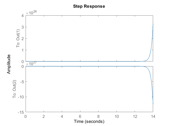
Open-loop cart position (top) and pendulum angle (bottom) in simulation for a voltage step input. The angle diverges, consistent with the unstable eigenvalue.
Pole Placement and Gain Matrix
Full state feedback closes the loop by setting the motor input u = r − Kx, where r is the reference input and K is a 1×4 gain row vector. The closed-loop system matrix becomes AK = A − BK, and its eigenvalues are placed anywhere in the left half plane by choosing K appropriately.
I computed the closed-loop characteristic polynomial as a function of the four gains k1 through k4 and matched its coefficients to a desired characteristic polynomial corresponding to a chosen set of stable closed-loop poles. Solving the resulting system of linear equations and verifying with MATLAB's place() function gave:
The characteristic polynomial of the desired closed-loop system is:
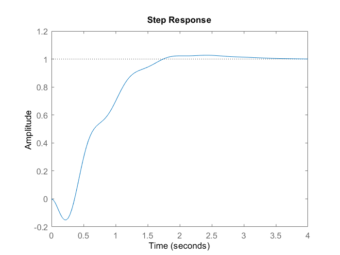
Simulated closed-loop step response of cart position to a 1 V reference input. The position converges smoothly to the commanded value.
I also simulated the tracking behavior under sinusoidal position references at 1, 2, and 5 rad/s, computing the ratio of output amplitude to input amplitude at each frequency:
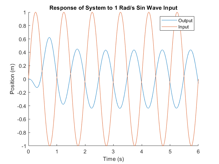
Simulation: cart tracking a 1 rad/s sine wave reference. Gain = 0.43.
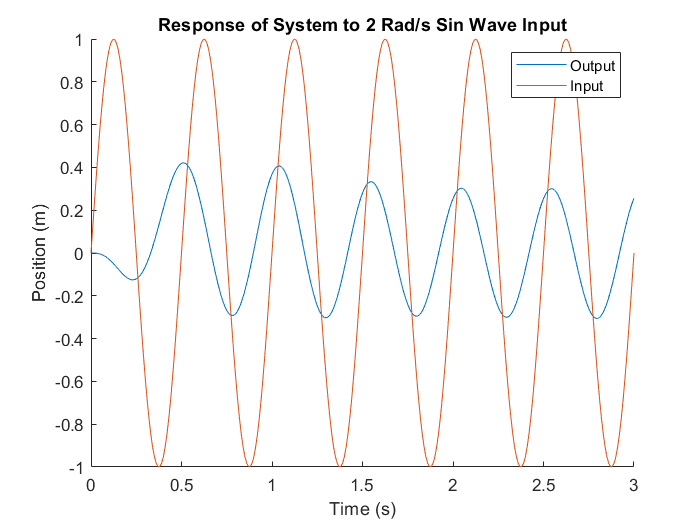
Simulation: 2 rad/s. Gain drops to 0.30 as frequency increases.
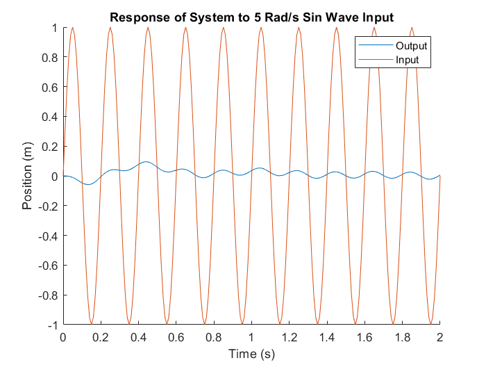
Simulation: 5 rad/s. Gain is 0.053, showing significant attenuation.
Hardware Implementation
I implemented the controller in Simulink with hardware-in-the-loop, using the physical cart-pendulum system with encoder measurements. The block diagram connected the gain matrix K to the real-time state measurements coming off the hardware encoders.
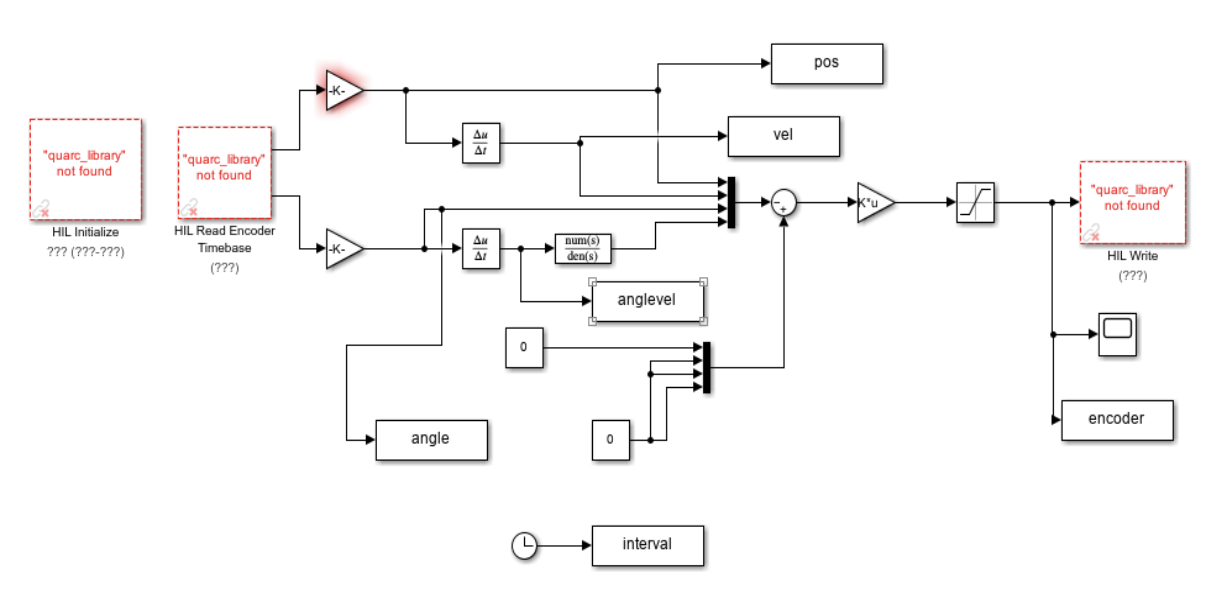
Simulink hardware model of the state feedback controller connected to the physical cart-pendulum system.
When connected with the pendulum in the upright position and given manual perturbations, the controller responded by driving the cart in the direction of the perturbation, counteracting the angular deviation and restoring the upright equilibrium. The pendulum remained stable through repeated pushes.
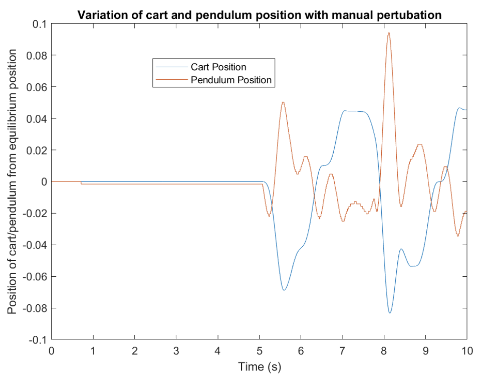
Hardware response to two manual perturbations. The spikes in pendulum angle show each push; the controller recovers quickly each time.
I tested the hardware controller against sinusoidal position references at the same three frequencies. The measured gains were consistently larger than the simulated ones, likely because the physical actuators and friction introduce dynamics not captured in the linear model:
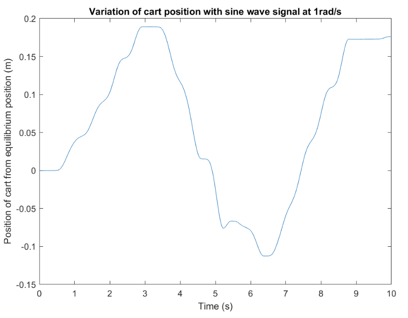
Hardware: cart position at 1 rad/s. Hardware gain (1.89) is much larger than the simulated prediction (0.43).
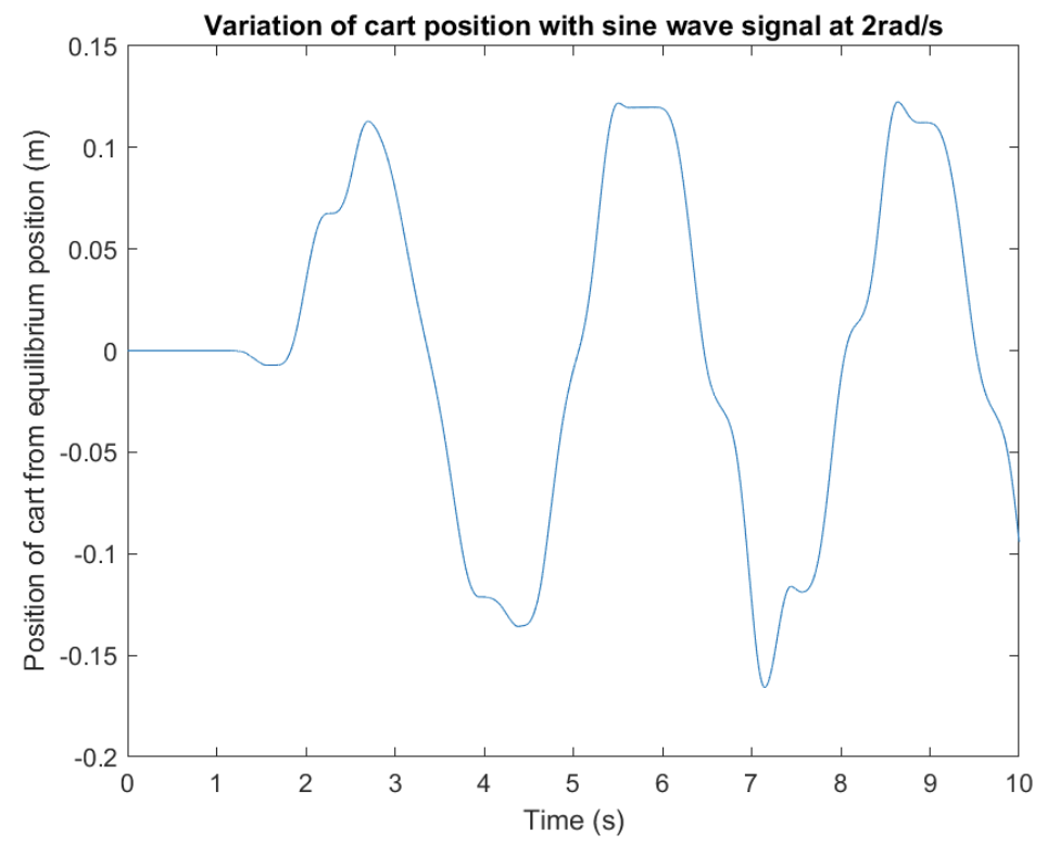
Hardware: cart position at 2 rad/s. Gain = 1.21 vs. simulated 0.30.
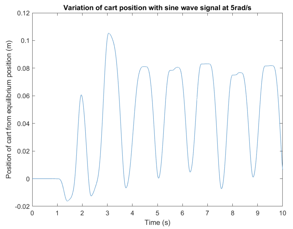
Hardware: cart position at 5 rad/s. Gain = 0.40 vs. simulated 0.053.
The Problem with Numerical Differentiation
The state vector includes ẋ and θ̇, which are not directly measured. In the first version of the controller, I estimated velocities by numerically differentiating the encoder position signals. Numerical differentiation amplifies high-frequency noise because each derivative computation effectively multiplies the noise spectrum by frequency. The resulting velocity signals contained large spikes that degraded control quality and caused jitter at higher reference frequencies.
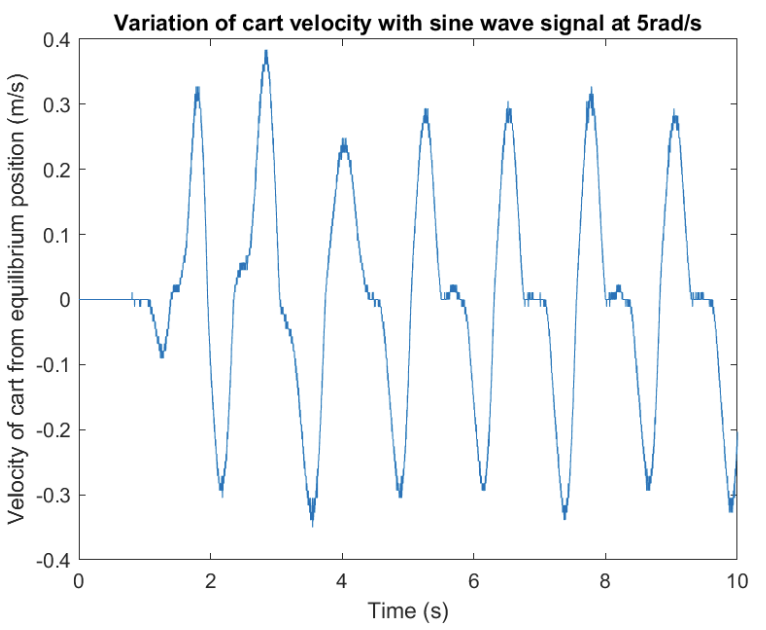
Cart velocity obtained by differentiating the cart position encoder at 5 rad/s. The noise is severe.
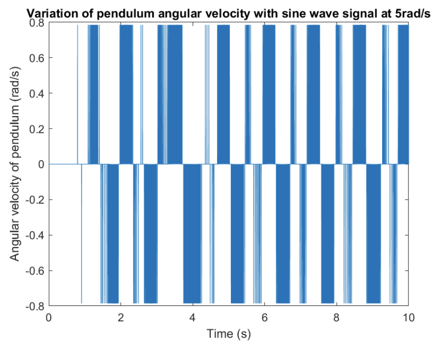
Pendulum angular velocity from differentiation. The high-frequency peaks reach amplitudes far exceeding the actual motion, making the signal nearly unusable.
Luenberger Observer Design
The solution is a Luenberger observer: a parallel model of the system that runs in software alongside the real plant, receiving the same input u and the measured outputs y, and correcting its state estimate x̂ based on the difference between predicted and measured outputs. The observer dynamics are:
The matrix L is a 4×2 observer gain matrix chosen so that the eigenvalues of (A − LC) are stable and converge faster than the closed-loop plant poles. I placed the observer eigenvalues at −10 ± 15j and −12 ± 17j, using MATLAB's place() command on the transposed system (place(A', C', poles)') to compute L:
[14.898 −2.248]
[240.608 7.676]
[15.343 22.290]
[179.300 403.180]
Because the observer poles lie further into the left half-plane than the controller poles, the observer converges to the actual state faster than the plant responds to control inputs. The observer provides smooth, noise-filtered estimates of all four states, including the velocities that were previously contaminated by differentiation noise.
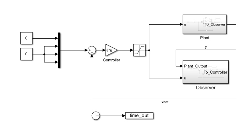
Overall Simulink model showing the controller, plant, and observer running in closed loop.
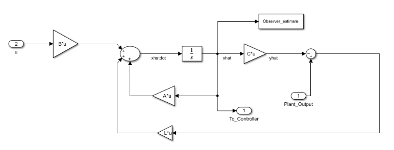
The observer block: it receives u and y, integrates the model forward, and feeds back L times the output error to correct the state estimate.
Observer Verification in Simulation
I simulated the observer starting from a mismatched initial condition (10 cm position offset, 5-degree angle offset in the plant, zero initial estimate). The observer estimate converged to the true plant state within roughly half a second across all four state variables:
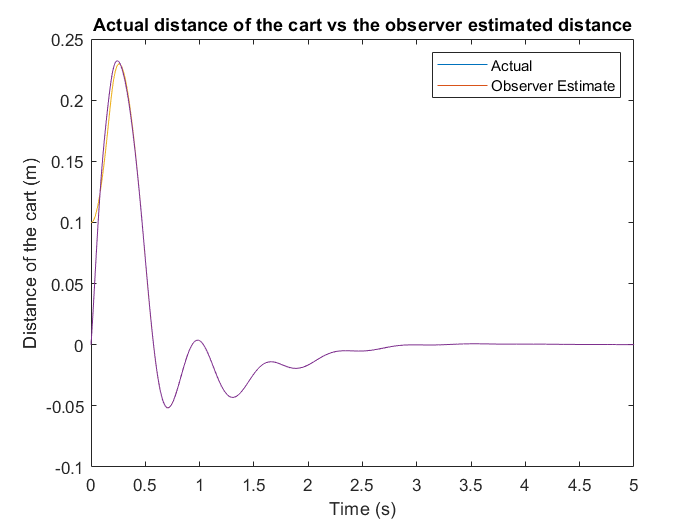
Cart position: actual (blue) vs observer estimate (orange). The observer converges quickly from the initial 10 cm offset.
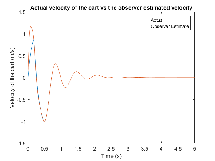
Cart velocity: the observer provides a smooth estimate without the noise spikes from numerical differentiation.
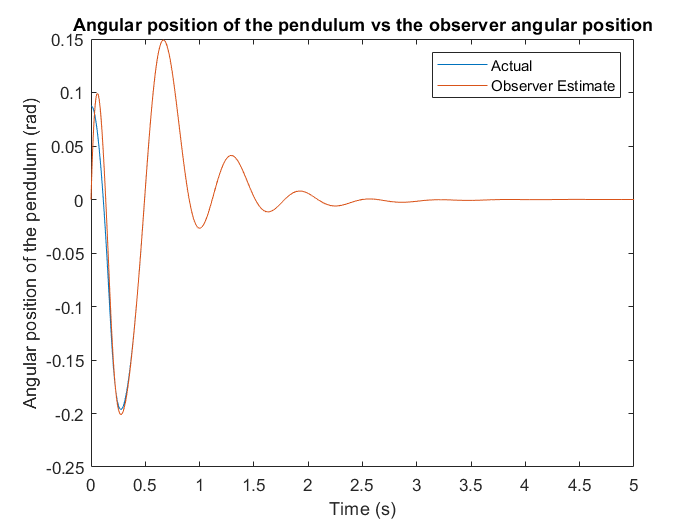
Pendulum angle: actual vs observer estimate. Error reduces to near zero before 0.5 seconds.
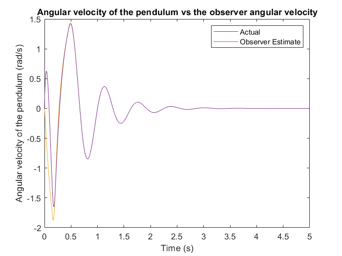
Pendulum angular velocity: the observer provides the smoothest estimate of the most noise-sensitive state.
Plotting the estimation error e = x̂ − x confirms rapid convergence:
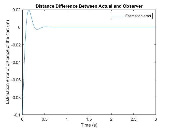
Position estimation error decays to near zero within half a second.
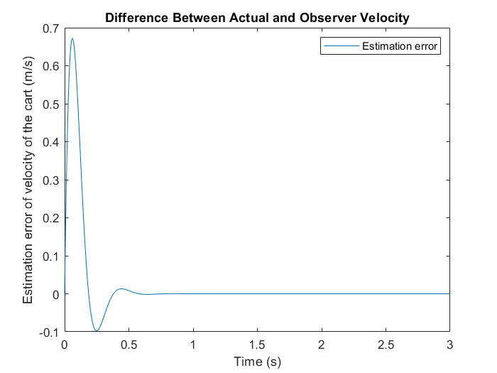
Velocity estimation error converges at the same rate as position error.
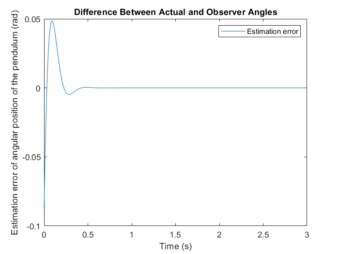
Angle estimation error. All four errors converge together, controlled by the observer eigenvalue placement.
Hardware: Observer vs Derivative Control
I ran both controllers on the physical hardware and compared their behavior. The observer-based controller produced visibly smoother cart and pendulum motion, especially during and after perturbations. When a perturbation was applied, the differentiation-based controller (Lab 6a) showed jagged, high-frequency activity in both cart position and pendulum angle. The observer-based controller responded more cleanly, with the estimate absorbing the noise before it reached the feedback path.
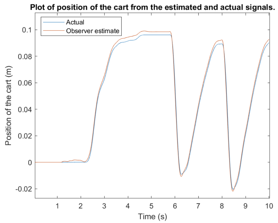
Hardware: observer estimate of cart position (orange) overlaid on the measured position (blue). The estimate closely tracks the actual signal.
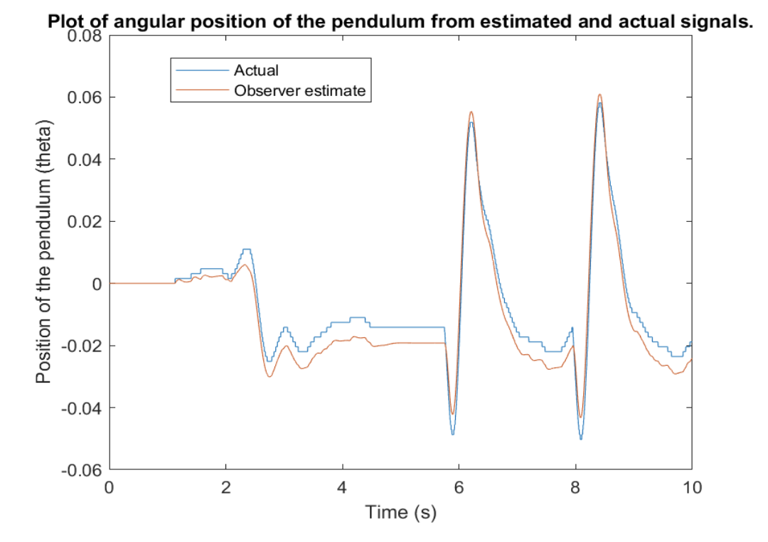
Hardware: observer estimate of pendulum angle vs measured angle. The observer provides a clean estimate even when the sensor signal carries encoder quantization noise.
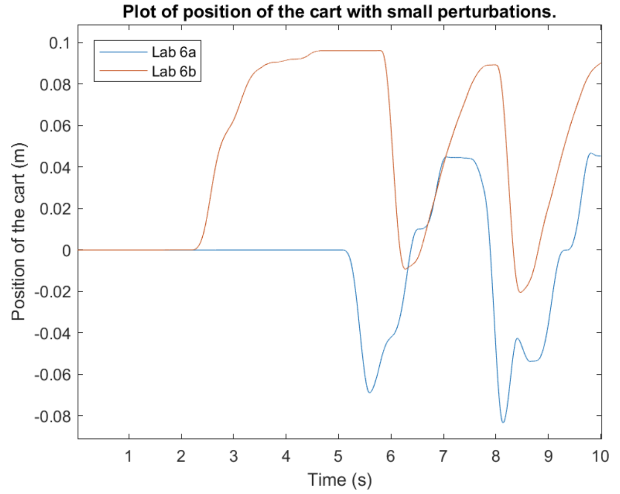
Cart position under perturbation: derivative-based controller (Lab 6a) vs observer-based controller (Lab 6b). The observer controller responds more smoothly.
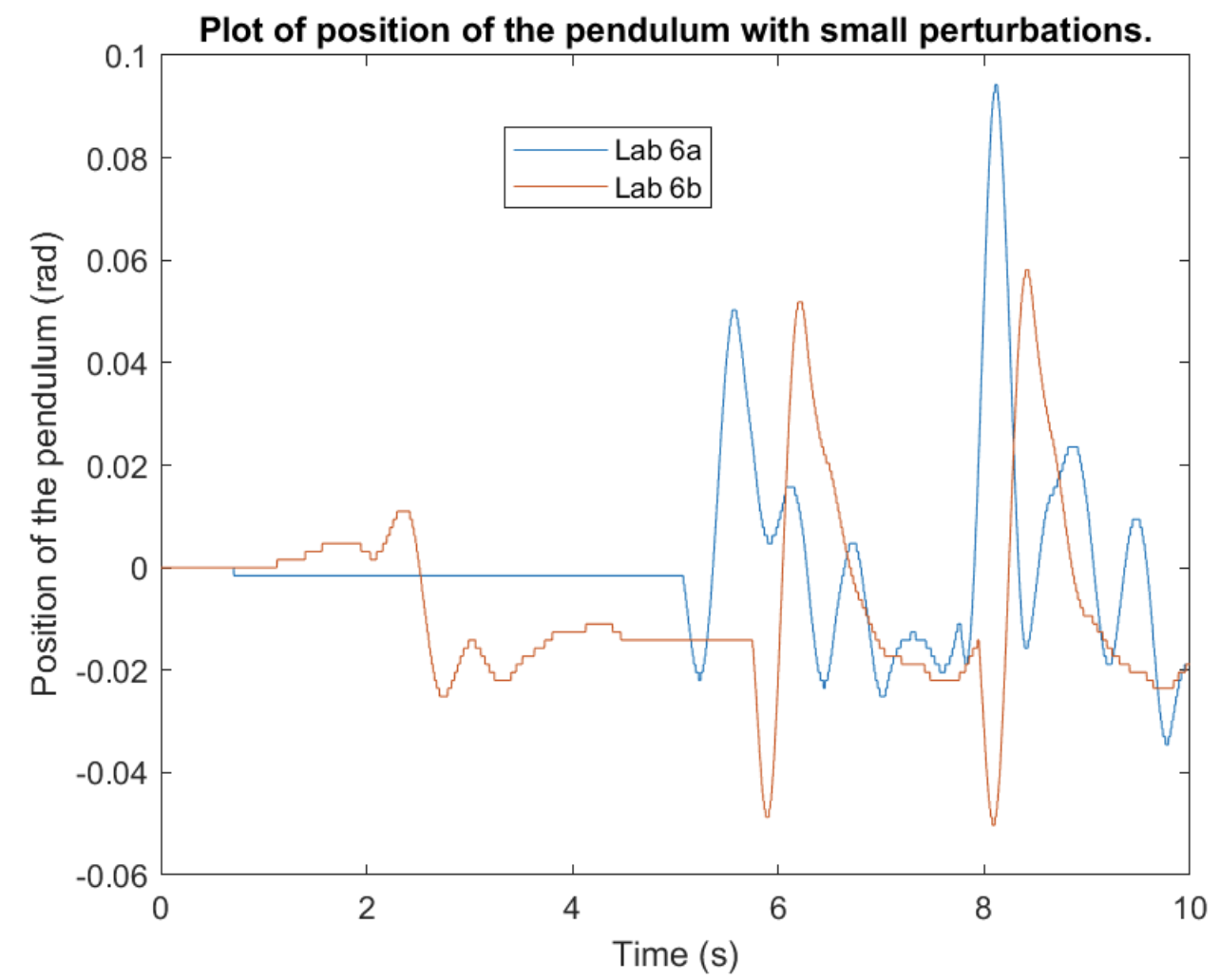
Pendulum angle under perturbation. The observer-based response is less jagged after the perturbation.
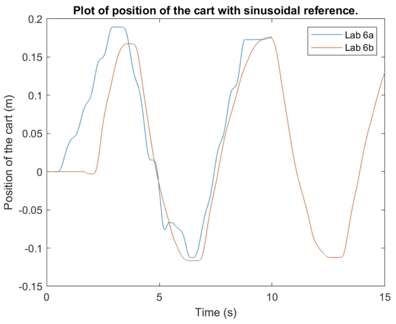
Cart position tracking a 1 rad/s sinusoidal reference: derivative controller (Lab 6a) vs observer controller (Lab 6b). The observer version tracks more smoothly.
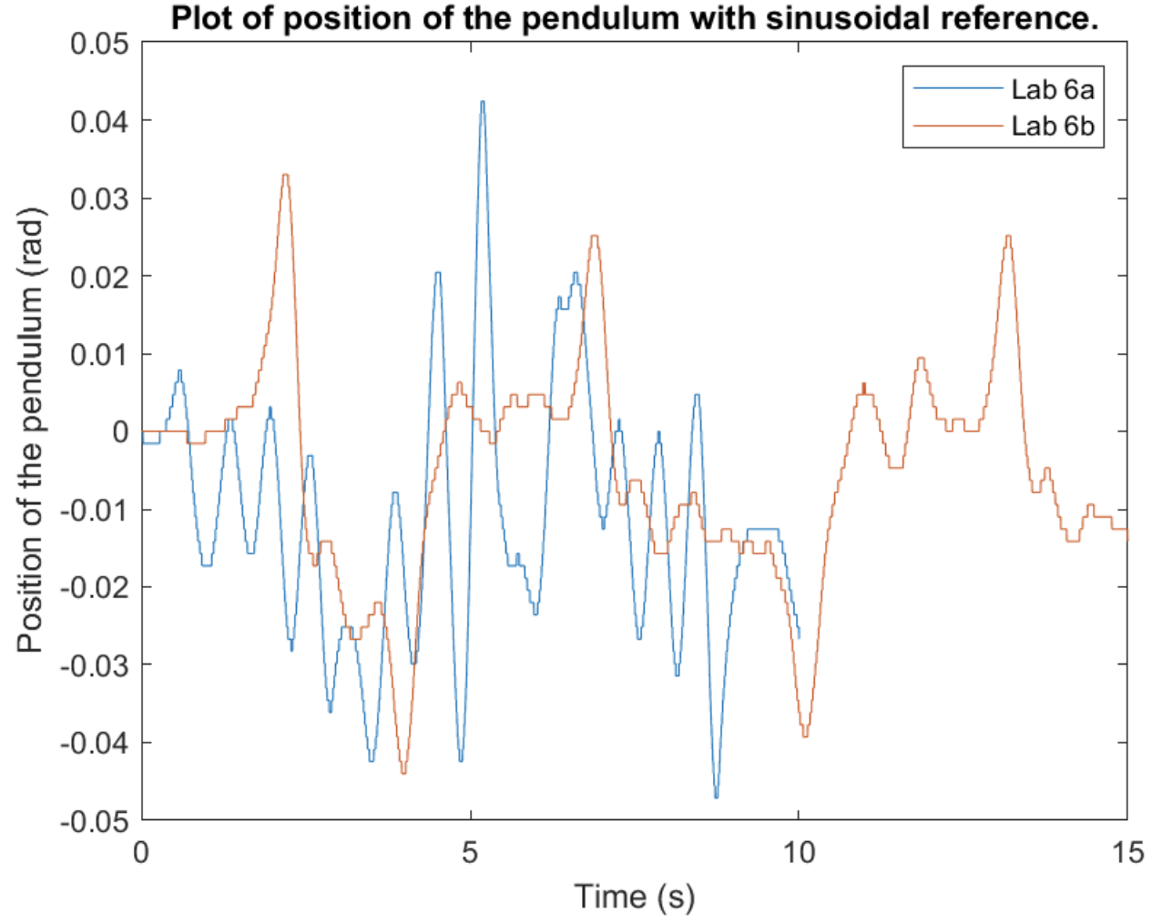
Pendulum angle during sine tracking. The observer controller keeps the pendulum angle tighter around zero while the cart moves.
The velocity comparison most clearly shows the advantage of the observer. Numerical differentiation introduced large noise peaks in the cart velocity and angular velocity signals. The observer replaced these with smooth, physically plausible estimates that the controller could act on without amplifying noise into the feedback loop:
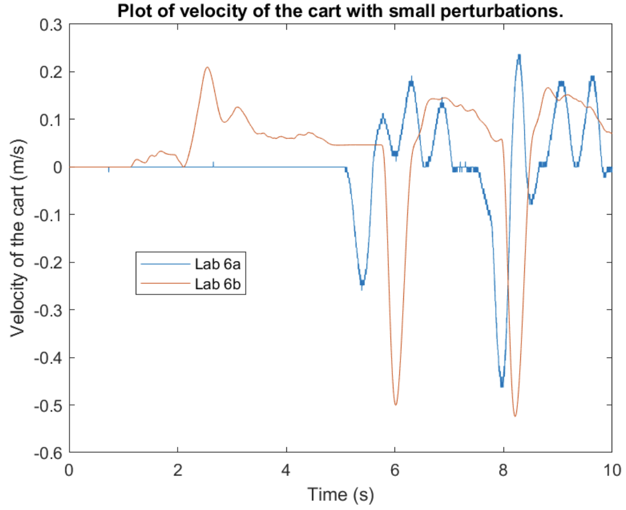
Cart velocity: derivative (Lab 6a, noisy) vs observer estimate (Lab 6b, smooth). The derivative version amplifies sensor noise into large spikes.
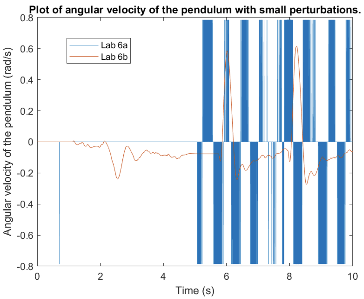
Pendulum angular velocity: the derivative signal has large high-frequency peaks that the observer entirely eliminates.
Noise Robustness Analysis
To quantify the observer's noise rejection, I ran an experiment with added measurement noise and compared three signals: the clean position, the noisy sensor output, and the observer estimate. I computed position deviation and noise power as performance metrics.
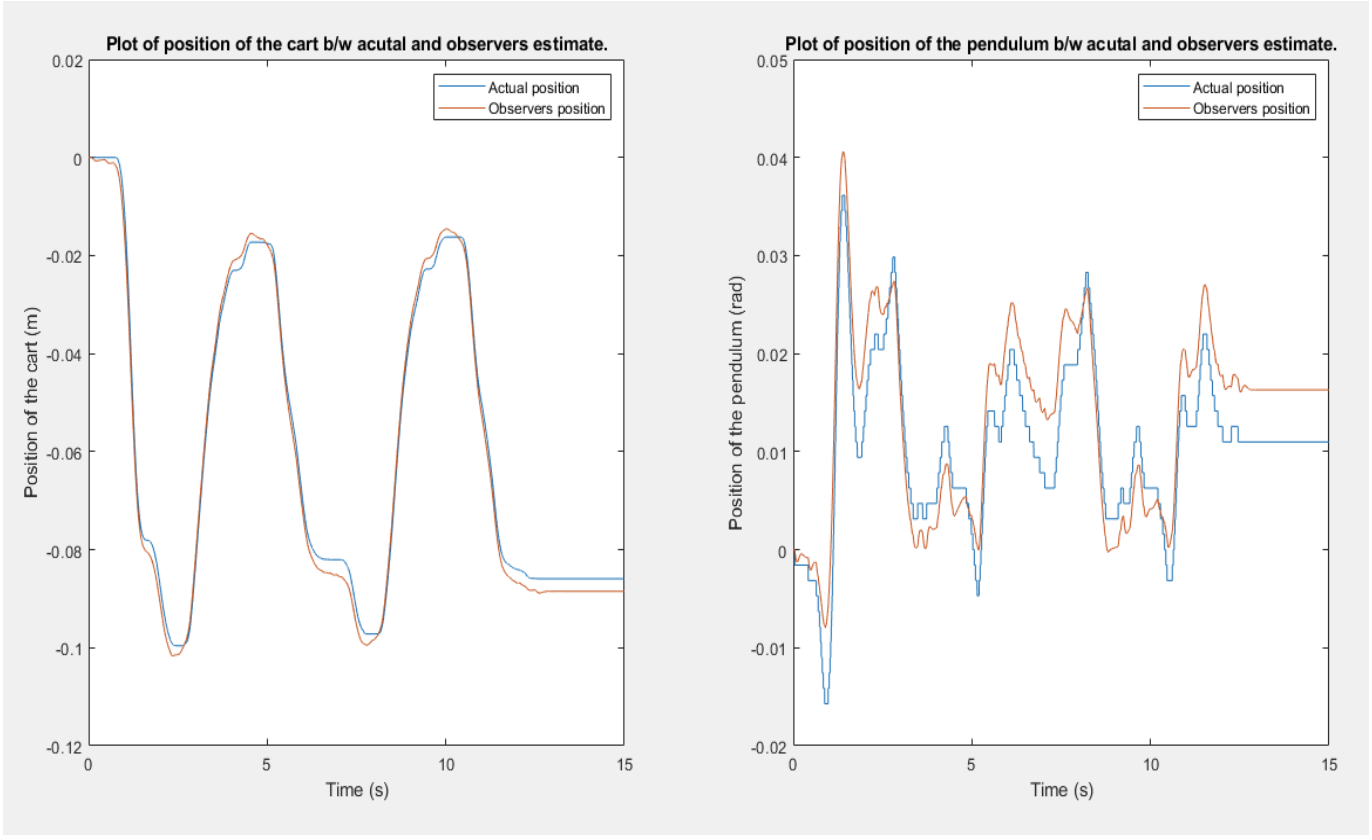
Observer noise test: actual and estimated cart position (top) and pendulum angle (bottom) plotted together. The observer estimate closely tracks the actual state despite sensor noise.
When I injected artificial noise into the sensor signals, the observer estimate remained close to the true state while the raw sensor output showed significant jitter. The position deviation and noise power metrics confirmed the observer was filtering effectively. I also explored three alternative pole placements to understand the tradeoffs between convergence speed and noise sensitivity. Poles placed closer to the real axis (smaller imaginary component) resulted in lower noise power while maintaining similar position deviation, suggesting that the pole imaginary parts primarily drive transient oscillation rather than steady-state noise rejection.
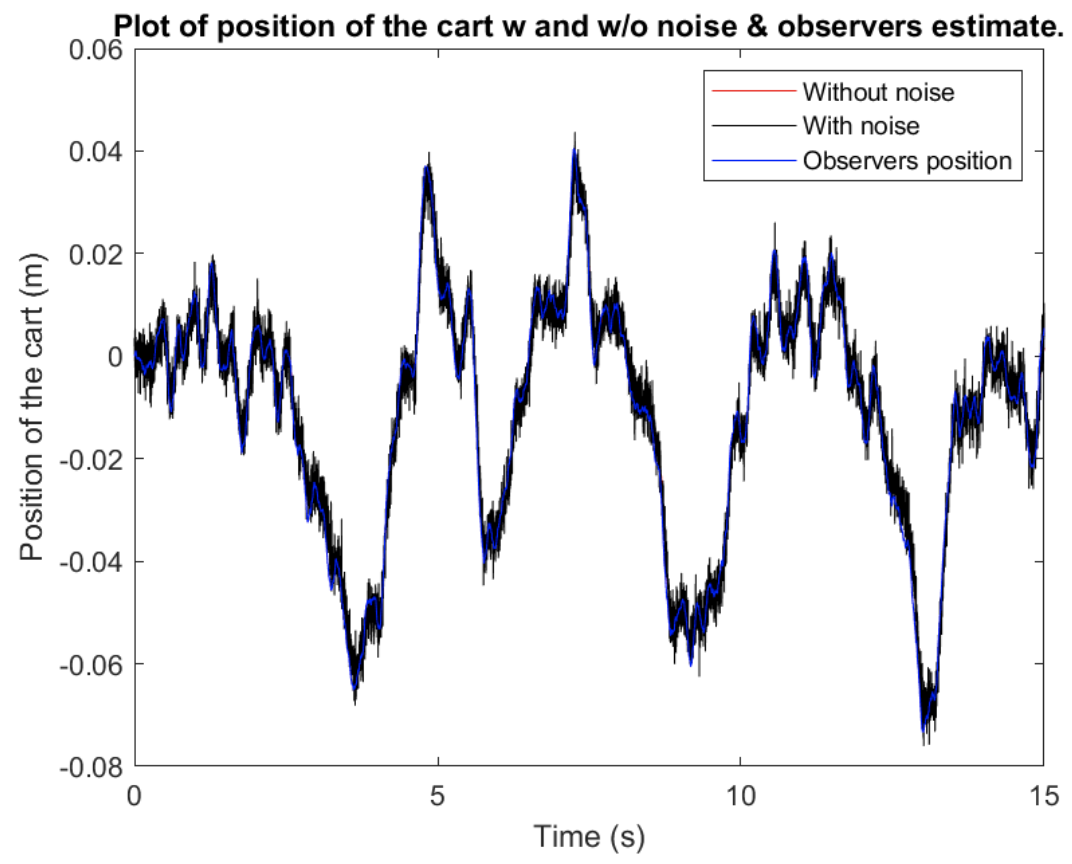
Cart position: clean signal (blue), noisy measurement (black), and observer estimate (red). The observer tracks the clean signal rather than the noisy one.
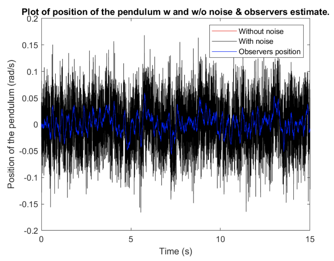
Pendulum angle under added noise. Angular noise power is much higher (0.84) than cart noise power (0.012), but the observer handles both.